Plot waveform and spectrum for a click

This function constructs and plots the waveform and spectrum for a click for which extra information has been recorded (IPI and SPL values for up to 21 cycles). By default, FPODs collect extra data for about 1% of detected clicks.

Usage

fp_plot(x, click_no = NULL, legend.pos = "topleft")

Arguments

x: A list object, as returned from fp_read().
click_no: integer. The click number. If NULL, then all clicks are plotted, in sequential order, one at a time.
legend.pos: character/logical. If character; a single keyword specifying the legend position. This parameter is passed as x when calling legend(). See legend() for details. If legend.pos is logical and FALSE, then the legend is suppressed.

Value

Invisibly returns a numeric vector with the frequency values used for plotting

Details

According to the FPOD software guide, extra data are stored for a small percentage of clicks (about 1%). The clicks to record are selected by a "real-time train detection algorithm" running on the FPOD. The information stored is the amplitude and timing (at 250 nanosecond resolution) of the peak of the soundwave. This allows for the reconstruction of the waveform by fitting sine waves to the points stored.

Note that there's an option in the FPOD app to configure the FPOD to record all clicks rather than just a small sample..

Examples

# read a FP3 file
fn <- fp_example("gullars_period1.FP3")
dat <- fp_read(fn)

# get the click number of the first five clicks for which we have WAV data.
first5 <- head(unique(dat$wav$click_no))

# plot one of them. Here, we plot number three
fp_plot(dat, first5[3])


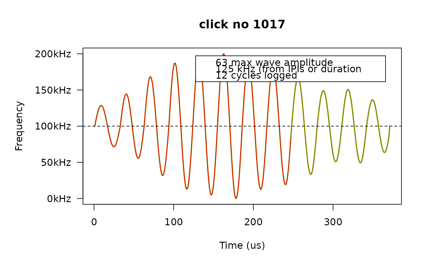
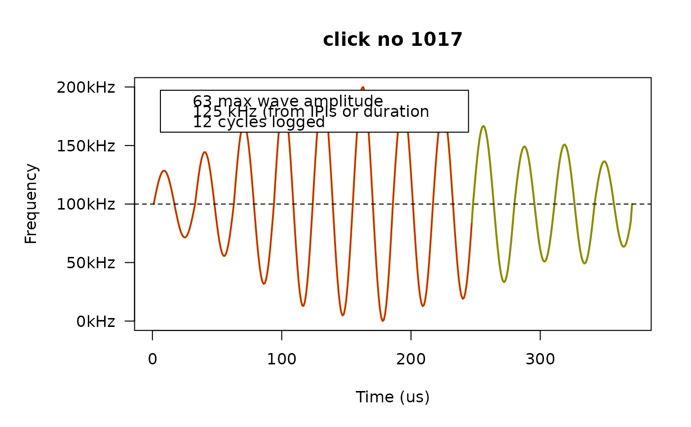# If the legend covers the curve, we can move it somewhere else.
fp_plot(dat, first5[3], legend.pos = "topright")


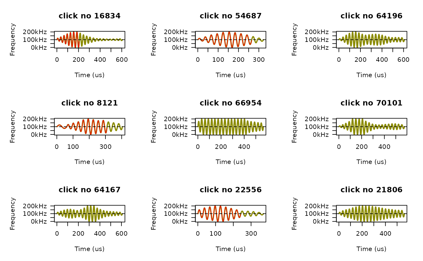
# If we only want to plot clicks that meet certain criteria, we have to do that
# manually. For example, we can plot 9 random NBHF clicks:
nbhf_clicks <- dat$clicks[species == "NBHF" & has_wav == TRUE, click_no]
old.mfrow = par()$mfrow
par(mfrow = c(3,3)) # we'll do 3 by 3 panels
for (i in sample(nbhf_clicks, size = 9)) {
    fp_plot(dat, click_no = i, legend.pos = FALSE)
}

par(mfrow = old.mfrow) # reset graphics device to whatever it was before